dlt & BigQuery Graph: From Raw Tables to Conversational Analytics in One Afternoon
In previous blogs we talked about how to build canonical models. This blog takes that further: we declare a BigQuery property graph over those models, query it with GQL, then ask it questions in plain English. The ontology resolved in the first step is what makes the answers right at the end.

Roshni Melwani
Working Student
6 min read
BigQuery shipped a native property-graph layer this year — CREATE PROPERTY GRAPH, GQL, zero data movement — and last month Conversational Analytics went GA, letting you ask that graph questions in plain English. Both are genuinely new. So we built the obvious demo: ingest a real relational dataset with dlt, turn it into clean canonical tables, declare a property graph over it, and see what happens when you ask it questions.
The short version: it works, and it works because the canonical layer was clean before the graph ever got declared. That's the actual point of this post.
The stack, in one line
dlt (ingest + canonical modeling) → CREATE PROPERTY GRAPH (BigQuery's structural graph layer) → Conversational Analytics (Gemini-powered natural language on top). Three tools, three different jobs, one pipeline.
Step 1 — Ingest
We pulled Chinook, a small but genuinely relational sample dataset (customers, employees, invoices, tracks, albums, artists, genres, playlists — real foreign keys, real multi-entity structure) straight into BigQuery with dlt's sql_database source:
import dlt
from dlt.sources.sql_database import sql_database

source = sql_database("sqlite:///chinook.db", schema="main")

pipeline = dlt.pipeline(
    pipeline_name="chinook_to_bq",
    destination="bigquery",
    dataset_name="roshni_bq_graph_demo",
)

load_info = pipeline.run(source)
A snapshot of how the data looks in BQ:
Eleven tables, fully typed, in BigQuery in under 30 seconds. No connector config beyond a connection string — dlt's schema inference did the rest.
Step 2 — Canonical tables
We previously explained in detail why you need a canonical model here, and we offer a guided process to model your data with LLMs + dlthub into a canonical model, read more here.
Chinook's raw tables are already reasonably normalized, so "canonical" here means: clear, purpose-built views with just the columns each entity needs, ready to become graph nodes and edges. We built these as plain BigQuery views, not copies — free to create, zero extra storage:
CREATE OR REPLACE VIEW `project.dataset.canonical_customer` AS
SELECT customer_id, first_name, last_name, email, city, country, support_rep_id
FROM `project.dataset.customers`;
(...one per entity: employee, invoice, track, album, artist, genre, playlist, plus two junction views for the many-to-many relationships.)
This is the step that matters most and gets the least airtime in most graph tutorials. A property graph is only as trustworthy as the tables underneath it — garbage in, garbage traversed.
Step 3 — Declare the graph
With clean canonical tables in place, the graph declaration is almost anticlimactic:
CREATE OR REPLACE PROPERTY GRAPH `project.dataset.chinook_graph`
NODE TABLES (
  canonical_customer KEY(customer_id) LABEL Customer,
  canonical_employee KEY(employee_id) LABEL Employee,
  canonical_invoice  KEY(invoice_id)  LABEL Invoice,
  canonical_track    KEY(track_id)    LABEL Track,
  canonical_album    KEY(album_id)    LABEL Album,
  canonical_artist   KEY(artist_id)   LABEL Artist,
  canonical_genre    KEY(genre_id)    LABEL Genre,
  canonical_playlist KEY(playlist_id) LABEL Playlist
)
EDGE TABLES (
  canonical_invoice AS placed
    KEY(invoice_id)
    SOURCE KEY(customer_id) REFERENCES canonical_customer(customer_id)
    DESTINATION KEY(invoice_id) REFERENCES canonical_invoice(invoice_id)
    LABEL Placed,
  canonical_invoice_contains_track AS invoice_purchased_track
    KEY(invoice_line_id)
    SOURCE KEY(invoice_id) REFERENCES canonical_invoice(invoice_id)
    DESTINATION KEY(track_id) REFERENCES canonical_track(track_id)
    LABEL Purchased,
  canonical_track AS recorded_on
    KEY(track_id)
    SOURCE KEY(track_id) REFERENCES canonical_track(track_id)
    DESTINATION KEY(album_id) REFERENCES canonical_album(album_id)
    LABEL RecordedOn,
  canonical_album AS performed_by
    KEY(album_id)
    SOURCE KEY(album_id) REFERENCES canonical_album(album_id)
    DESTINATION KEY(artist_id) REFERENCES canonical_artist(artist_id)
    LABEL PerformedBy
  -- ...plus SupportedBy, ReportsTo, HasGenre, Includes (each with its own KEY() too)
)
Zero data movement — the graph is a schema declaration over tables that already exist. Eight node types, eight edges, built in one DDL statement.
Here’s the snapshot of the graph produced:
Three gotchas worth flagging if you're following along:
- Every node and edge table needs its own explicit
KEY()— not just theSOURCE KEY/DESTINATION KEYjoin columns. Skip it and BigQuery errors with "must have primary key defined." - Table references inside
CREATE PROPERTY GRAPHneed fullproject.dataset.tablequalification — no default-dataset inference like a normal query gets. CONTAINSis a reserved SQL keyword — you can't use it unquoted as an edge alias or label. (We renamed ours toPurchased.)
Step 4 — Query it with GQL
Here's the traversal we ended up asking in production: find every artist a given customer has bought music from — a 4-hop path (Customer → Invoice → Track → Album → Artist).
The SQL version of "find everything reachable within N hops" is a recursive CTE — a base case, a recursive step, a manual visited-array to stop cycles, DISTINCT at the end to dedupe. The GQL version is one MATCH clause that reads like the sentence you'd say out loud:
GRAPH chinook_graph
MATCH (c:Customer)-[:Placed]->(i:Invoice)-[:Purchased]->(t:Track)
      -[:RecordedOn]->(al:Album)-[:PerformedBy]->(ar:Artist)
WHERE c.customer_id = 1
RETURN DISTINCT c.first_name, c.last_name, ar.name AS artist_name
No manual JOINs, no recursion to hand-write. That's the actual argument for a native graph layer on relationship-shaped questions — not that SQL can't do it, but that you stop having to write traversal logic by hand.
Step 5 — Ask it in English
This is where it gets interesting. We pointed BigQuery's Conversational Analytics (via Agent Catalog) at chinook_graph and asked, in plain English:
"Which artists has customer Luís Gonçalves purchased tracks from?"
The agent answered correctly — 15 artists — and the GQL it wrote on its own, unprompted, was clean and correct:
GRAPH `dlthub-sandbox.roshni_bq_graph_demo.chinook_graph`
MATCH (c:Customer WHERE c.first_name = 'Luís' AND c.last_name = 'Gonçalves')
      -[:Placed]->(i:Invoice)
      -[:Purchased]->(t:Track)
      -[:RecordedOn]->(al:Album)
      -[:PerformedBy]->(art:Artist)
RETURN DISTINCT art.name AS artist_name
ORDER BY artist_name
It found the full 4-hop path and picked the right edge labels straight from the schema — no hints, no examples, no hand-holding. Then it went further than the literal question, unprompted, surfacing "Analysis Insights" (diverse musical taste, a distinct Brazilian-music preference) and three smart follow-up questions.
The detail that makes the whole argument
While setting up the agent, we found the real evidence for why the canonical layer matters. Every Conversational Analytics agent has an Instructions field — and Google's own placeholder examples for it read like this:
"Never use these fields: Transaction Date Derived, City Derived."
"For any question about date grouping, use Order Date unless another field is specified."
"For questions about 'transaction value' use the column 'Derived eCommerce Transaction Value' and not 'Transaction Amount.'"
That's a human, manually, agent-side, patching ambiguity the schema alone can't resolve — which column actually means what the business means. It's exactly the problem dlt's ontology and canonical-modeling work solves upstream, before data ever reaches a graph or an agent. Even Google's own tool needs a slot to inject business meaning — it just puts that slot at the very end of the pipeline (per-agent, hand-typed) instead of the beginning (once, in your canonical model, inherited by everything downstream).
Our agent never needed an Instructions field. It didn't need one because the ambiguity had already been resolved two steps earlier, when the canonical tables were built.
And this isn't just an analogy — it's wireable. Conversational Analytics reads BigQuery table and column descriptions as schema context (Google's own docs recommend adding them for accuracy). That means dlt's ontology-resolved business meaning could be written directly onto the canonical tables as column descriptions, and the agent would pick it up automatically — no one hand-typing an Instructions field per agent. dlt's ontology becomes the metadata; the agent just reads it.
Takeaway
Ontology isn't one layer, it's a stack:
- dlt's layer (upstream): what does this data mean? A Customer is a Customer, an Invoice is a purchase event, a Track belongs to an Album which belongs to an Artist — resolved once, in code, before anything downstream has to guess.
- BigQuery's layer (downstream): how do I expose those meanings as something traversable at scale?
CREATE PROPERTY GRAPHturns clean tables into nodes and edges with zero data movement. - Conversational Analytics (the interface): ask it in English, get a correct answer and the query that produced it.
Skip the first layer and the second two don't catch the mistake — they just build a structurally valid graph, or a fluent English answer, on top of a business model that's quietly wrong. dlt builds the ontology; BigQuery serves it.
Call to action
If you’re on bigquery, give it a shot! it’s an impressive feature! If you’re not on BigQuery, we offer a dltHub blueprint for conversational analytics.