Access loaded data in Python

This guide explains how to access and manipulate data that has been loaded into your destination using the dlt Python library. After running your pipelines and loading data, you can use the pipeline.dataset() and data frame expressions, Ibis or SQL to query the data and read it as records, Pandas frames or Arrow tables.

Quick start example

Here's a full example of how to retrieve data from a pipeline and load it into a Pandas DataFrame or a PyArrow Table.

# Assuming you have a Pipeline object named 'pipeline'. You can create one with the dlt cli: dlt init fruitshop duckdb
# and you have loaded the data of the fruitshop example source into the destination
# the tables available in the destination are:
# - customers
# - inventory
# - purchases

# Step 1: Get the readable dataset from the pipeline
dataset = pipeline.dataset()

# Step 2: Access a table as a ReadableRelation
customers_relation = dataset.table("customers")

# Step 3: Fetch the entire table as a Pandas DataFrame
df = customers_relation.df()  # or customers_relation.df(chunk_size=50)

# Alternatively, fetch as a PyArrow Table
arrow_table = customers_relation.arrow()

Getting started

Assuming you have a Pipeline object (let's call it pipeline), you can obtain a Dataset which contains the credentials and schema to your destination dataset. You can construct a query and execute it on the dataset to retrieve a Relation which you may use to retrieve data from the Dataset.

Note: The Dataset and Relation objects are lazy-loading. They will only query and retrieve data when you perform an action that requires it, such as fetching data into a DataFrame or iterating over the data. This means that simply creating these objects does not load data into memory, making your code more efficient.

Access the dataset

# Get the readable dataset from the pipeline
dataset = pipeline.dataset()

# print the row counts of all tables in the destination as dataframe
print(dataset.row_counts().df())

Access tables as dataset

The simplest way of getting a Relation from a Dataset is to get a full table relation:

# Using `table` method`
customers_relation = dataset.table("customers")

# Using item access
customers_relation = dataset["customers"]

Creating relations with sql query strings

# Join 'customers' and 'purchases' tables and filter by quantity
query = """
SELECT *  
    FROM customers 
JOIN purchases 
    ON customers.id = purchases.customer_id
WHERE purchases.quantity > 1
"""
joined_relation = dataset(query)

Reading data

Once you have a Relation, you can read data in various formats and sizes.

Fetch the entire table

warning

Loading full tables into memory without limiting or iterating over them can consume a large amount of memory and may cause your program to crash if the table is too large. It's recommended to use chunked iteration or apply limits when dealing with large datasets.

As a Pandas DataFrame

df = customers_relation.df()

As a PyArrow Table

arrow_table = customers_relation.arrow()

As a list of Python tuples

items_list = customers_relation.fetchall()

Lazy loading behavior

The Dataset and Relation objects are lazy-loading. This means that they do not immediately fetch data when you create them. Data is only retrieved when you perform an action that requires it, such as calling .df(), .arrow(), or iterating over the data. This approach optimizes performance and reduces unnecessary data loading.

Iterating over data in chunks

To handle large datasets efficiently, you can process data in smaller chunks.

Iterate as Pandas DataFrames

for df_chunk in customers_relation.iter_df(chunk_size=5):
    # Process each DataFrame chunk
    pass

Iterate as PyArrow Tables

for arrow_chunk in customers_relation.iter_arrow(chunk_size=5):
    # Process each PyArrow chunk
    pass

Iterate as lists of tuples

for items_chunk in customers_relation.iter_fetch(chunk_size=5):
    # Process each chunk of tuples
    pass

The methods available on the Relation correspond to the methods available on the cursor returned by the SQL client. Please refer to the SQL client guide for more information.

Connection Handling

For every call that actually fetches data from the destination, such as df(), arrow(), fetchall() etc., the dataset will open a connection and close it after it has been retrieved or the iterator is completed. You can keep the connection open for multiple requests with the dataset context manager:

# the dataset context manager will keep the connection open
# and close it after the with block is exited
with dataset:
    print(dataset.table("customers").limit(50).arrow())
    print(dataset.table("purchases").arrow())

Special queries

You can use the row_counts method to get the row counts of all tables in the destination as a DataFrame.

# print the row counts of all tables in the destination as dataframe
print(dataset.row_counts().df())

# or as tuples
print(dataset.row_counts().fetchall())

Modifying queries

You can refine your data retrieval by limiting the number of records, selecting specific columns, sorting the results, filtering rows, aggregating minimum and maximum values on a specific column, or chaining these operations.

Limit the number of records

# Get the first 50 items as a PyArrow table
arrow_table = customers_relation.limit(50).arrow()

Using head() to get the first 5 records

df = customers_relation.head().df()

Select specific columns

# Select only 'id' and 'name' columns
items_list = customers_relation.select("id", "name").fetchall()

# Alternate notation with brackets
items_list = customers_relation[["id", "name"]].fetchall()

# Only get one column
items_list = customers_relation[["name"]].fetchall()

Sort results

# Order by 'id'
ordered_list = customers_relation.order_by("id").fetchall()

Filter rows

# Filter by 'id'
filtered = customers_relation.where("id", "in", [3, 1, 7]).fetchall()

# Filter with raw SQL string
filtered = customers_relation.where("id = 1").fetchall()

# Filter with sqlglot expression
import sqlglot.expressions as sge

expr = sge.EQ(
    this=sge.Column(this=sge.to_identifier("id", quoted=True)),
    expression=sge.Literal.number("7"),
)
filtered = customers_relation.where(expr).fetchall()

Aggregate data

# Get max 'id'
max_id = customers_relation.select("id").max().fetchscalar()

# Get min 'id'
min_id = customers_relation.select("id").min().fetchscalar()

Join related tables

Use join() to navigate dlt's schema references between related tables, such as parent/child tables created from nested data, or tables where you explicitly annotate the relationship. Joined columns are prefixed with the joined table name, or with the alias you provide.

users_with_orders = dataset["users"].join("users__orders", alias="orders")
df = users_with_orders.select("name", "orders__order_id", "orders__total").df()

Chain operations

You can combine select, limit, and other methods.

# Select columns and limit the number of records
arrow_table = customers_relation.select("id", "name").limit(50).arrow()

Modifying queries with ibis expressions

If you install the amazing ibis library, you can use ibis expressions to modify your queries.

pip install ibis-framework

dlt will then allow you to get an ibis.Table for each table which you can use to build a query with ibis expressions, which you can then execute on your dataset.

warning

A previous version of dlt allowed to use ibis expressions in a slightly different way, allowing users to directly execute and retrieve data on ibis Unbound tables. This method does not work anymore. See the migration guide below for instructions on how to update your code.

# now that ibis is installed, we can get ibis unbound tables from the dataset
dataset = pipeline.dataset()

# get two table expressions
customers_expression = dataset.table("customers").to_ibis()
purchases_expression = dataset.table("purchases").to_ibis()

# join them using an ibis expression
join_expression = customers_expression.join(
    purchases_expression,
    customers_expression.id == purchases_expression.customer_id,
)

# now we can use the ibis expression to filter the data
filtered_expression = join_expression.filter(purchases_expression.quantity > 1)

# we can pass the expression back to the dataset to get a relation that can be executed
relation = dataset(filtered_expression)
# and we can inspect the query that will be used to read the data
print(relation)

# and finally fetch the data as a pandas dataframe, the same way we would do with a normal relation
print(relation.df())

# a few more examples

# get all customers from berlin and london and load them as a dataframe
expr = customers_expression.filter(
    customers_expression.city.isin(["berlin", "london"])
)
print(dataset(expr).df())

# limit and offset, then load as an arrow table
expr = customers_expression.limit(10, offset=5)
print(dataset(expr).arrow())

# mutate columns by adding a new colums that always is 10 times the value of the id column
expr = customers_expression.mutate(new_id=customers_expression.id * 10)
print(dataset(expr).df())

# sort asc and desc
import ibis

expr = customers_expression.order_by(ibis.desc("id"), ibis.asc("city")).limit(10)
print(dataset(expr).df())

# group by and aggregate
expr = (
    customers_expression.group_by("city")
    .having(customers_expression.count() >= 3)
    .aggregate(sum_id=customers_expression.id.sum())
)
print(dataset(expr).df())

# subqueries
expr = customers_expression.filter(
    customers_expression.city.isin(["berlin", "london"])
)
print(dataset(expr).df())

You can learn more about the available expressions on the ibis for sql users page.

Migrating from the previous dlt / ibis implementation

As describe above, the new way to use ibis expressions is to first get one or many Table objects and construct your expression. Then, you can pass it Dataset to get a Relation to execute the full query and retrieve data.

An example from our previous docs for joining a customers and a purchase table was this:

# get two relations
customers_relation = dataset["customers"]
purchases_relation = dataset["purchases"]

# join them using an ibis expression
joined_relation = customers_relation.join(
    purchases_relation, customers_relation.id == purchases_relation.customer_id
)

# ... do other ibis operations

# directly fetch the data on the expression we have built
df = joined_relation.df()

The migrated version looks like this:

# we convert the dlt.Relation an Ibis Table object
customers_expression = dataset.table("customers").to_ibis()
purchases_expression = dataset.table("purchases").to_ibis()

# join them using an ibis expression, same code as above
joined_epxression = customers_expression.join(
    purchases_expression, customers_expression.id == purchases_expression.customer_id
)

# ... do other ibis operations, would be same as before

# now convert the expression to a relation
joined_relation = dataset(joined_epxression)

# execute as before
df = joined_relation.df()

Supported destinations

All SQL and filesystem destinations supported by dlt can utilize this data access interface.

Reading data from filesystem

For filesystem destinations, dlt uses DuckDB under the hood to create views on iceberg and delta tables or from Parquet, JSONL and csv files. This allows you to query data stored in files using the same interface as you would with SQL databases. If you plan on accessing data in buckets or the filesystem a lot this way, it is advised to load data into delta or iceberg tables, as DuckDB is able to only load the parts of the data actually needed for the query to work.

tip

By default dlt will not autorefresh views created on iceberg tables and files when new data is loaded. This prevents wasting resources on file globbing and reloading iceberg metadata for every query. You can change this behavior with always_refresh_views flag.

Note: delta tables are by default on autorefresh which is implemented by delta core and seems to be pretty efficient.

Examples

Fetch one record as a tuple

record = customers_relation.fetchone()

Fetch many records as tuples

records = customers_relation.fetchmany(10)

Iterate over data with limit and column selection

Note: When iterating over filesystem tables, the underlying DuckDB may give you a different chunk size depending on the size of the parquet files the table is based on.

# Dataframes
for df_chunk in (
    customers_relation.select("id", "name").limit(100).iter_df(chunk_size=20)
):
    ...

# Arrow tables
for arrow_table in (
    customers_relation.select("id", "name").limit(100).iter_arrow(chunk_size=20)
):
    ...

# Python tuples
for records in (
    customers_relation.select("id", "name").limit(100).iter_fetch(chunk_size=20)
):
    # Process each modified DataFrame chunk
    ...

Advanced usage

Loading a Relation into a pipeline table

Since the iter_arrow and iter_df methods are generators that iterate over the full Relation in chunks, you can use them as a resource for another (or even the same) dlt pipeline:

# Create a readable relation with a limit of 1m rows
limited_customers_relation = dataset.customers.limit(1_000_000)

# Create a new pipeline
other_pipeline = dlt.pipeline(pipeline_name="other_pipeline", destination="duckdb")

# We can now load these 1m rows into this pipeline in 10k chunks
other_pipeline.run(
    limited_customers_relation.iter_arrow(chunk_size=10_000),
    table_name="limited_customers",
)

Learn more about transforming data in Python with Arrow tables or DataFrames.

Datasets with multiple schemas

When a pipeline loads data from several sources, each source produces its own schema. By default, all schemas share one physical dataset and pipeline.dataset() includes every schema automatically, so tables from all sources are queryable together. If two schemas define a table with the same name, dlt merges their columns and combines rows from both — missing columns are filled with NULL.

note

Multi-schema datasets are not recommended for most use cases. They arise naturally when multiple sources are loaded into one pipeline, and dlt handles them transparently. You can restrict the dataset to a single schema with pipeline.dataset(schema="source_name") or pass a list of schemas to select a subset. Load history is tracked per schema — use dataset.load_ids(schema_name="...") to query a specific one.

Breaking changes

Breaking changes introduced in dlt 1.25.0

The following changes affect existing code that uses pipeline.dataset():

pipeline.dataset() now includes all schemas by default. Previously, calling pipeline.dataset() without a schema argument returned only the default schema's tables. Now, when use_single_dataset is enabled (the default) and the pipeline has multiple schemas, all schemas are included automatically. Code that assumed only one schema's tables are visible may now see additional tables or extra rows in shared table names. To restore the previous single-schema behavior, pass the schema explicitly:

# Before (implicit single schema):
ds = pipeline.dataset()

# After (explicit single schema, equivalent to the old behavior):
ds = pipeline.dataset(schema=pipeline.default_schema_name)

Staging dataset

So far, we've been using the append write disposition in our example pipeline. This means that each time we run the pipeline, the data is appended to the existing tables. When you use the merge write disposition, dlt creates a staging database schema for staging data. This schema is named <dataset_name>_staging by default and contains the same tables as the destination schema. When you run the pipeline, the data from the staging tables is loaded into the destination tables in a single atomic transaction.

Let's illustrate this with an example. We change our pipeline to use the merge write disposition:

import dlt

@dlt.resource(primary_key="id", write_disposition="merge")
def users():
    yield [
        {'id': 1, 'name': 'Alice 2'},
        {'id': 2, 'name': 'Bob 2'}
    ]

pipeline = dlt.pipeline(
    pipeline_name='quick_start',
    destination='duckdb',
    dataset_name='mydata'
)

load_info = pipeline.run(users)

Running this pipeline will create a schema in the destination database with the name mydata_staging. If you inspect the tables in this schema, you will find the mydata_staging.users table identical to the mydata.users table in the previous example.

Here is what the tables may look like after running the pipeline:

mydata_staging.users

id	name	_dlt_id	_dlt_load_id
1	Alice 2	wX3f5vn801W16A	2345672350.98417
2	Bob 2	rX8ybgTeEmAmmA	2345672350.98417

mydata.users

id	name	_dlt_id	_dlt_load_id
1	Alice 2	wX3f5vn801W16A	2345672350.98417
2	Bob 2	rX8ybgTeEmAmmA	2345672350.98417
3	Charlie	h8lehZEvT3fASQ	1234563456.12345

Notice that the mydata.users table now contains the data from both the previous pipeline run and the current one.

dev_mode (versioned datasets)

When you set the dev_mode argument to True in the dlt.pipeline call, dlt creates a versioned dataset. This means that each time you run the pipeline, the data is loaded into a new dataset (a new database schema). The dataset name is the same as the dataset_name you provided in the pipeline definition with a datetime-based suffix.

We modify our pipeline to use the dev_mode option to see how this works:

import dlt

data = [
    {'id': 1, 'name': 'Alice'},
    {'id': 2, 'name': 'Bob'}
]

pipeline = dlt.pipeline(
    pipeline_name='quick_start',
    destination='duckdb',
    dataset_name='mydata',
    dev_mode=True # <-- add this line
)
load_info = pipeline.run(data, table_name="users")

Every time you run this pipeline, a new schema will be created in the destination database with a datetime-based suffix. The data will be loaded into tables in this schema. For example, the first time you run the pipeline, the schema will be named mydata_20230912064403, the second time it will be named mydata_20230912064407, and so on.

Internal dlt tables

dlt automatically creates internal tables in the destination schema to track pipeline runs, support incremental loading, and manage schema versions. These tables use the _dlt_ prefix.

_dlt_loads

This table records each pipeline run. Every time you execute a pipeline, a new row is added to this table with a unique load_id. This table tracks which loads have been completed and supports chaining of transformations.

Column name	Type	Description
load_id	STRING	Unique identifier for the load job
schema_name	STRING	Name of the schema used during the load
schema_version_hash	STRING	Hash of the schema version
status	INTEGER	Load status. Value 0 means completed
inserted_at	TIMESTAMP	When the load was recorded

Only rows with status = 0 are considered complete. Other values represent incomplete or interrupted loads. The status column can also be used to coordinate multi-step transformations.

_dlt_pipeline_state

This table stores the internal state of the pipeline for each run. This state enables incremental loading and allows the pipeline to resume from where it left off if a previous run was interrupted.

Column name	Type	Description
version	INTEGER	Version of this state entry
engine_version	INTEGER	Version of the dlt engine used
pipeline_name	STRING	Name of the pipeline
state	STRING or BLOB	Serialized Python dictionary of pipeline state
created_at	TIMESTAMP	When this state entry was created
version_hash	STRING	Hash to detect changes in the state
_dlt_load_id	STRING	Reference to related load in _dlt_loads
_dlt_id	STRING	Unique identifier for the pipeline state row

The state column contains a serialized Python dictionary that includes:

• Incremental progress (e.g. last item or timestamp processed).
• Checkpoints for transformations.
• Source-specific metadata and settings.

This allows dlt to resume interrupted pipelines, avoid reloading already processed data, and ensure pipelines are idempotent and efficient.

The version_hash is recalculated on each update. dlt uses this table to implement last-value incremental loading. If a run fails or stops, this table ensures the next run picks up from the correct checkpoint.

_dlt_version

This table tracks the history of all schema versions used by the pipeline. Every time dlt updates the schema. For example, when new columns or tables are added, a new entry is written to this table.

Column name	Type	Description
version	INTEGER	Numeric version of the schema
engine_version	INTEGER	Version of the dlt engine used
inserted_at	TIMESTAMP	Time the schema version entry was created
schema_name	STRING	Name of the schema
version_hash	STRING	Unique hash representing the schema content
schema	STRING or JSON	Full schema in JSON format

By keeping previous schema definitions, _dlt_version ensures that:

• Older data remains readable
• New data uses updated schema rules
• Backward compatibility is maintained

This table also supports troubleshooting and compatibility checks. It lets you track which schema and engine version were used for any load. This helps with debugging and ensures safe evolution of your data model.

Ibis

Ibis is a powerful portable Python dataframe library. Learn more about what it is and how to use it in the official documentation.

dlt provides an easy way to hand over your loaded dataset to an Ibis backend connection.

tip

Not all destinations supported by dlt have an equivalent Ibis backend. Natively supported destinations include DuckDB (including Motherduck), Postgres (Redshift is supported via the Postgres backend for Ibis versions lower than 10.4.0), Snowflake, Clickhouse, MSSQL (including Synapse), and BigQuery. The filesystem destination is supported via the Filesystem SQL client; please install the DuckDB backend for Ibis to use it. Mutating data with Ibis on the filesystem will not result in any actual changes to the persisted files.

Prerequisites

To use the Ibis backend, you will need to have the ibis-framework package with the correct Ibis extra installed. The following example will install the DuckDB backend:

pip install ibis-framework[duckdb]

Get an Ibis connection from your dataset

dlt datasets have a helper method to return an Ibis connection to the destination they live on. The returned object is a native Ibis connection to the destination, which you can use to read and even transform data. Please consult the Ibis documentation to learn more about what you can do with Ibis.

Breaking change in dlt 1.25.0

dataset.ibis() now passes all schemas from the dataset to the Ibis backend. On filesystem destinations, this means Ibis will see tables from every schema in the dataset and not just the default one. If two schemas define the same table name, the Ibis table will contain rows from both schemas combined. To get the previous single-schema behavior, create the dataset with an explicit schema: pipeline.dataset(schema="my_schema").ibis().

# get the dataset from the pipeline
dataset = pipeline.dataset()
dataset_name = pipeline.dataset_name

# get the native ibis connection from the dataset
ibis_connection = dataset.ibis()

# list all tables in the dataset
# NOTE: You need to provide the dataset name to ibis, in ibis datasets are named databases
print(ibis_connection.list_tables(database=dataset_name))

# get the items table
table = ibis_connection.table("items", database=dataset_name)

# print the first 10 rows
print(table.limit(10).execute())

# Visit the ibis docs to learn more about the available methods

Marimo

marimo is a reactive Python notebook. It completely revamps the Jupyter notebook experience. Whenever code is executed or you interact with a UI element, dependent cells are re-executed ensuring consistency between code and displayed outputs.

This page shows how dlt + marimo + ibis provide a rich environment to explore loaded data, write data transformations, and create data applications.

Prerequisites

To install marimo and ibis with the duckdb extras, run the following command:

pip install marimo "ibis-framework[duckdb]"

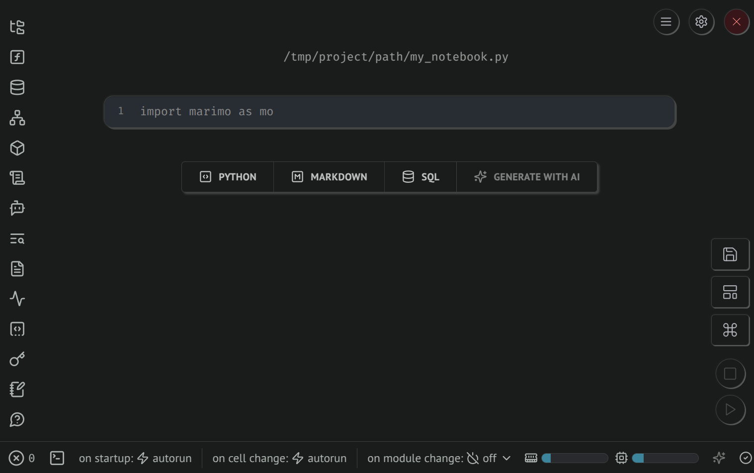
Launch marimo

Use this command to launch marimo (replace my_notebook.py with desired name). It will print a link to access the notebook web app.

marimo edit my_notebook.py

> Edit my_notebook.py in your browser 📝
>   ➜  URL: http://localhost:2718?access_token=Qfo_Hj2RbXqiqM4VT3XOwA 

Here's a screenshot of the interface you should see:

Features

Use custom dlt widgets

Inside your marimo notebook, you can use composable widgets built and maintained by the dlt team. This requires the mowidgets package (Python 3.11+).

Import them from dlt.helpers.marimo and pass them to the render() function:

#%% cell 1
from dlt.helpers.marimo import render, load_package_viewer, pipeline_selector

#%% cell 2
render(pipeline_selector)

#%% cell 3
render(load_package_viewer, pipeline_path="/path/to/pipeline")

Available widgets: pipeline_selector, load_package_viewer, schema_viewer.

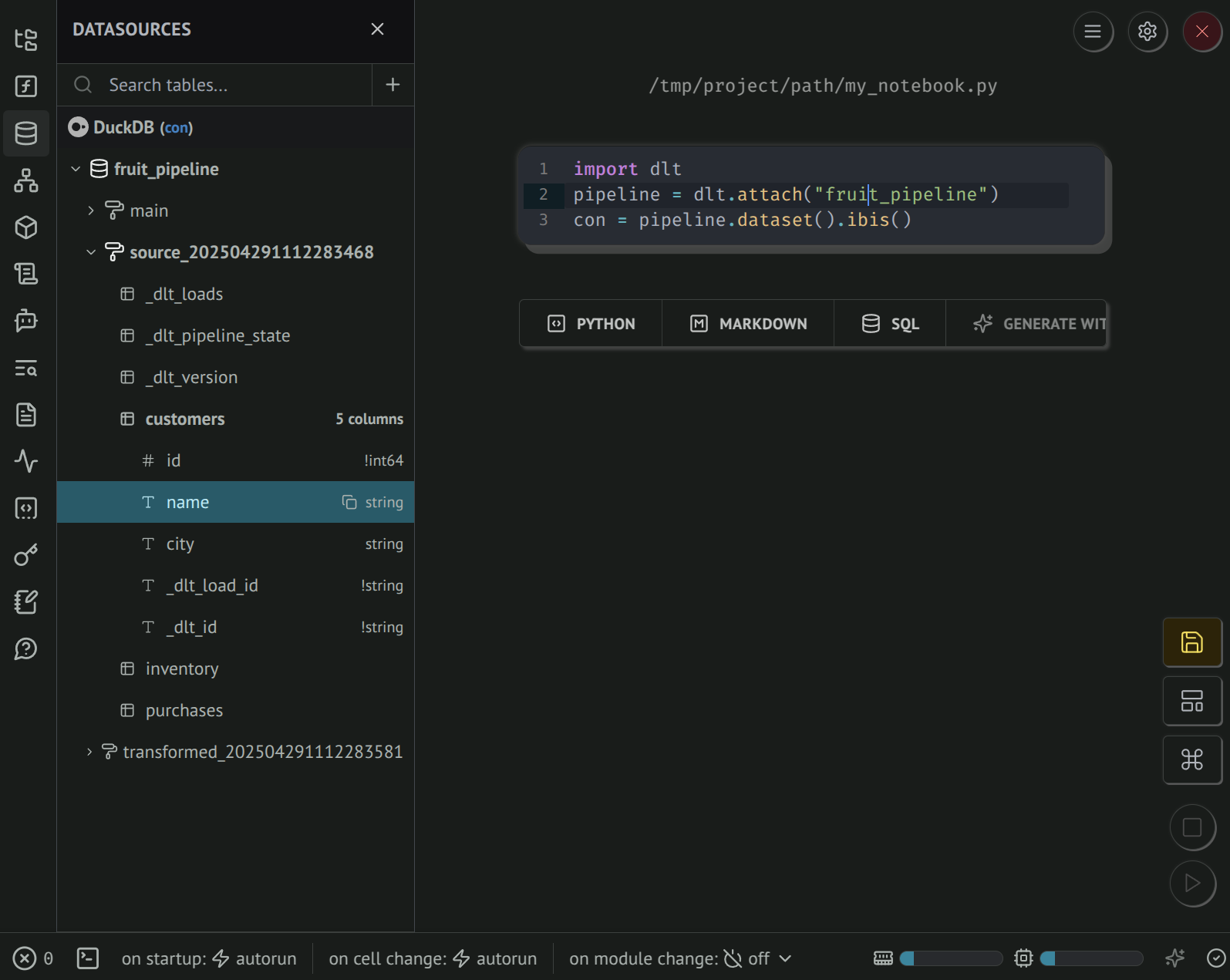
View dataset tables and columns

After loading data with dlt, you can access it via the dataset interface, including a native ibis connection.

In marimo, the Datasources panel provides a GUI to explore data tables and columns. When a cell contains a variable that's an ibis connection, it is automatically registered.

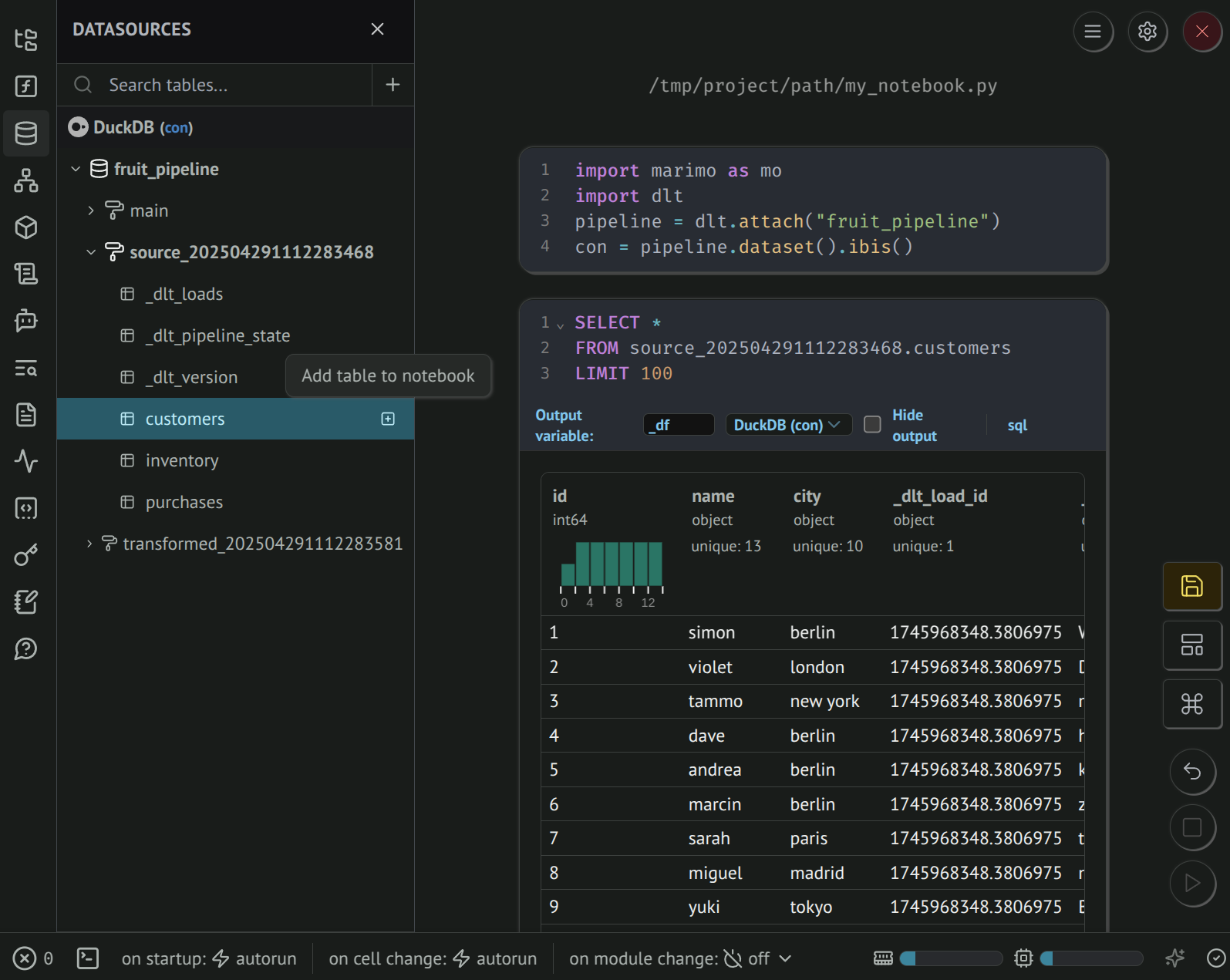
Accessing data with SQL

Clicking on the Add table to notebook button will create a new SQL cell that you can use to query data. The output cell provides a rich and interactive results dataframe.

note

The Datasources displays a limited range of data types.

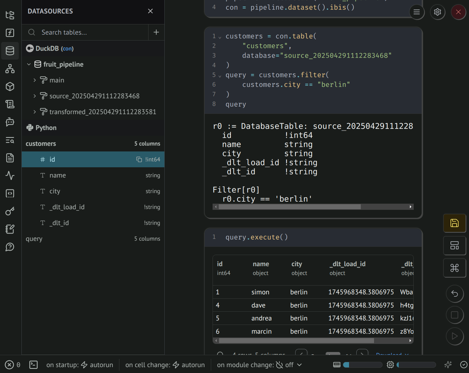
Accessing data with Python

You can also retrieve Ibis tables (lazy expressions) using Python. The Datasources panel will show under Python the output schema of your Ibis query, and the cell output will display detailed query planning.

Use .execute(), .to_pandas(), .to_polars(), or .to_pyarrow() to execute the Ibis expression and retrieve data that can displayed in a rich and interactive dataframe.

note

The Datasources displays a limited range of data types.

Create a dashboard and data apps

marimo notebooks can be deployed as web applications with interactive UI and charts and the code hidden. Try adding marimo UI input elements, rich markdown, and charts (matplotlib, plotly, altair, etc.). Combined, dlt + marimo + ibis make it easy to build a simple dashboard on top of fresh data.

Further reading

• Learn about marimo dataframe and SQL features
• Explore databases using the marimo GUI
• Learn about marimo if you're coming from Streamlit

Important considerations

• Memory usage: Loading full tables into memory without iterating or limiting can consume significant memory, potentially leading to crashes if the dataset is large. Always consider using limits or chunked iteration.

• Lazy evaluation: Dataset and Relation objects delay data retrieval until necessary. This design improves performance and resource utilization.

• Custom SQL queries: When executing custom SQL queries, remember that additional methods like limit() or select() won't modify the query. Include all necessary clauses directly in your SQL statement.