Version: devel View Markdown

Access loaded data in Python

This guide explains how to access and change data that dlt loaded into your destination. After a pipeline run, use pipeline.dataset() to query the data. You can build the query with data frame expressions, Ibis, or SQL. You can read the result as records, Pandas frames, or Arrow tables.

Quick start example

This example reads data from a pipeline into a Pandas DataFrame or a PyArrow Table.

# This example needs a Pipeline object named 'pipeline' with the fruitshop data loaded.
# Create one with: dlt init fruitshop duckdb
# the tables available in the destination are:
# - customers
# - inventory
# - purchases

# Step 1: Get the dataset from the pipeline
dataset = pipeline.dataset()

# Step 2: Access a table as a Relation
customers_relation = dataset.table("customers")

# Step 3: Read the entire table as a Pandas DataFrame
df = customers_relation.df()  # or customers_relation.df(chunk_size=50)

# Alternatively, read as a PyArrow Table
arrow_table = customers_relation.arrow()

Getting started

A Pipeline object gives you a Dataset, which holds the credentials and the schema of your destination dataset. Build a query on the dataset to get a Relation. The Relation reads the data.

Note: The Dataset and Relation objects defer their work. They query the destination only when you take an action that needs the data, for example a read into a DataFrame. See Deferred query execution.

Access the dataset

# Get the dataset from the pipeline
dataset = pipeline.dataset()

# print the row counts of all tables in the destination as a DataFrame
print(dataset.row_counts().df())

Access tables as relations

The simplest Relation is a full table:

# Using the `table` method
customers_relation = dataset.table("customers")

# Using bracket notation
customers_relation = dataset["customers"]

Create relations with SQL query strings

# Join 'customers' and 'purchases' tables and filter by quantity
query = """
SELECT *
    FROM customers
JOIN purchases
    ON customers.id = purchases.customer_id
WHERE purchases.quantity > 1
"""
joined_relation = dataset(query)

Reading data

Once you have a Relation, you can read data in various formats and sizes.

Fetch the entire table

warning

If a table is large, apply a limit or iterate in chunks. A full table read can exhaust memory and stop your program.

As a Pandas DataFrame

df = customers_relation.df()

As a PyArrow Table

arrow_table = customers_relation.arrow()

As a list of Python tuples

items_list = customers_relation.fetchall()

Deferred query execution

The Dataset and Relation objects read no data when you create them. The read happens when you take an action that needs the data, for example a call to .df() or .arrow(). An iteration over the relation also triggers the read. A relation you build but never read sends no query.

Iterating over data in chunks

To handle large datasets efficiently, you can process data in smaller chunks.

Iterate as Pandas DataFrames

for df_chunk in customers_relation.iter_df(chunk_size=5):
    # Process each DataFrame chunk
    pass

Iterate as PyArrow Tables

for arrow_chunk in customers_relation.iter_arrow(chunk_size=5):
    # Process each PyArrow chunk
    pass

Iterate as lists of tuples

for items_chunk in customers_relation.iter_fetch(chunk_size=5):
    # Process each chunk of tuples
    pass

The methods on the Relation match the methods on the cursor that the SQL client returns. See the SQL client guide.

Connection handling

Some calls read data from the destination, for example df(), arrow(), and fetchall(). For each of these calls, the dataset opens a connection. The dataset closes the connection after the read completes or the iterator ends. To keep one connection open across several calls, use the dataset context manager:

# the dataset context manager keeps the connection open
# and closes it when the with block ends
with dataset:
    print(dataset.table("customers").limit(50).arrow())
    print(dataset.table("purchases").arrow())

Special queries

You can use the row_counts method to get the row counts of all tables in the destination as a DataFrame.

# print the row counts of all tables in the destination as a DataFrame
print(dataset.row_counts().df())

# or as tuples
print(dataset.row_counts().fetchall())

Modifying queries

You can change a query in these ways:

limit the number of records
select specific columns
sort the results
filter rows
aggregate the minimum and maximum of a column
chain these operations

Limit the number of records

# Get the first 50 items as a PyArrow table
arrow_table = customers_relation.limit(50).arrow()

Using `head()` to get the first 5 records

df = customers_relation.head().df()

Select specific columns

# Select only 'id' and 'name' columns
items_list = customers_relation.select("id", "name").fetchall()

# Alternate notation with brackets
items_list = customers_relation[["id", "name"]].fetchall()

# Only get one column
items_list = customers_relation[["name"]].fetchall()

Sort results

# Order by 'id'
ordered_list = customers_relation.order_by("id").fetchall()

Filter rows

# Filter by 'id'
filtered = customers_relation.where("id", "in", [3, 1, 7]).fetchall()

# Filter with a raw SQL string
filtered = customers_relation.where("id = 1").fetchall()

# Filter with a sqlglot expression
import sqlglot.expressions as sge

expr = sge.EQ(
    this=sge.Column(this=sge.to_identifier("id", quoted=True)),
    expression=sge.Literal.number("7"),
)
filtered = customers_relation.where(expr).fetchall()

Aggregate data

# Get max 'id'
max_id = customers_relation.select("id").max().fetchscalar()

# Get min 'id'
min_id = customers_relation.select("id").min().fetchscalar()

Filter to an incremental cursor

Relation.incremental(incremental) adds a WHERE clause derived from a dlt.sources.incremental cursor so a relation only sees rows in the cursor window.

import dlt
from dlt.common.pendulum import pendulum

dataset = pipeline.dataset()

# bounded read: all rows in [2026-01-01, 2026-02-01)
cursor = dlt.sources.incremental(
    "created_at",
    initial_value=pendulum.datetime(2026, 1, 1, tz="UTC"),
    end_value=pendulum.datetime(2026, 2, 1, tz="UTC"),
)
rows = dataset.table("events").incremental(cursor).fetchall()

Or pass it directly on dataset.table(..., incremental=...):

rows = dataset.table("events", incremental=cursor).fetchall()

Relation.incremental() accepts cursor paths in two forms:

column — filters on a column of the relation's base table.
table.column — automatically joins table via the dataset schema and filters on the joined column. The joined table's columns are not added to the projection. If the same table is already joined, the existing join is reused.

Cursor on an auto-joined column

A dotted cursor_path of the form table.column auto-joins table and filters on the joined column. This form uses the same schema-reference resolution as Relation.join(). The dlt schema must connect table to the current relation's base table through parent/child references. dlt does not add the joined columns to the projection. dlt reuses an existing JOIN to the same table.

A common case is filtering any user table by dlt load time via _dlt_loads:

# only rows from loads that happened after 2026-01-01
cursor = dlt.sources.incremental(
    "_dlt_loads.inserted_at",
    initial_value=pendulum.datetime(2026, 1, 1, tz="UTC"),
)
events = dataset.table("events", incremental=cursor)

The translation from Incremental to SQL follows these rules:

last_value_func must be max or min. Custom callables can't be pushed down to SQL.
range_start / range_end decide endpoint inclusivity ("closed" -> >=/<=, "open" -> >/<). Operator direction follows last_value_func.
on_cursor_value_missing="include" translates to ... OR cursor IS NULL. "exclude" translates to ... AND cursor IS NOT NULL. "raise" cannot raise mid-query in SQL pushdown, so it falls back to IS NOT NULL. It emits a warning unless the schema marks the cursor column as not nullable.
dlt applies lag to the lower bound, exactly as it does during a resource extraction.

See Incremental transformations to use this in @dlt.hub.transformation. That page covers stateful cursors, scheduler-owned windows, and _dlt_loads.inserted_at load-time cursors.

The join() method appends a related table to the current relation. It works in two modes:

Auto-join via schema references: dlt builds the join condition from parent/child relationships dlt creates during loading, plus any references you declared on a resource.
Explicit on predicate: when you pass on=, you write the join condition yourself. Use it for any join the auto mode cannot do. This includes joins across two datasets in the same data location.

By default, join() creates an inner join. To choose another SQL join type, pass kind="left", "right", or "full".

Without an alias, joined columns take the target table name as their prefix. For example, dataset["users"].join("users__orders") adds columns such as users__orders__order_id. With alias="orders", the same column becomes orders__order_id. Pass an alias to shorten result column names or to avoid a name conflict.

Auto-join via schema references

With no on argument, join() follows relationships already defined in the dlt schema. It resolves direct schema references between tables. It also resolves multi-hop parent/child paths when one table is an ancestor or descendant of the other. The auto mode therefore suits nested tables that dlt created, and tables connected by explicit references. dlt appends columns from the target table only, under the target table name or the alias you provide.

users_with_orders = dataset["users"].join(
    "users__orders", alias="orders", kind="left"
)
df = users_with_orders.select("name", "orders__order_id", "orders__total").df()

The auto mode works on relations from dataset[name] or dataset.table(name). It also works on relations chained from them with where(), select(), order_by(), and similar methods. It does not work on relations from dataset.query("..."). For those relations, use the explicit form below.

The auto mode does not support:

arbitrary join conditions
joins on columns that you pick yourself
self-joins
joins across different datasets
joins between tables that are only related indirectly through a shared ancestor or another non-linear schema path

In practice, this means the auto mode supports ancestor/descendant navigation, but not general graph traversal across the schema:

dataset["users__orders__items"].join("users") works because users is an ancestor in the nested table hierarchy
two sibling tables that both descend from users do not join
two tables do not join on a custom predicate such as orders.customer_email = customers.email. Use the explicit form below.

The auto mode can need intermediate tables to build the path to the target table. dlt uses those tables for the path only. dlt appends columns from the joined target table alone.

Explicit join condition

Pass on= to write the join condition yourself, as a SQL string or a sqlglot expression. If the auto mode does not work for your tables, use this form. One example is a join between two top-level tables with no parent/child relationship.

# `customers` and `purchases` are two top-level tables connected
# by `purchases.customer_id` and `customers.id`. There is no schema
# reference between them, so we provide the join condition ourselves.
customers_with_purchases = dataset["customers"].join(
    "purchases",
    on="customers.id = purchases.customer_id",
    kind="left",
)

# the right-hand side can also be a transformed relation. dlt keeps its
# filters when it embeds the relation as a subquery.
big_purchases = dataset["purchases"].where("quantity", "gt", 3)
customers_with_big_purchases = dataset["customers"].join(
    big_purchases,
    on="customers.id = purchases.customer_id",
    alias="big",
)

df = customers_with_big_purchases.select("name", "big__id", "big__quantity").df()

The right-hand side can be a table name, a table relation, or a relation you already transformed with select() or where(). When you pass a transformed relation, its filters and column selection carry over to the joined result.

In on, refer to the right-hand side by its source qualifier. The qualifier is the joined table's name, or the alias you gave it in a dataset.query(...). Some relations have no identifiable source, for example a constant dataset.query("SELECT 1 AS id") with no FROM. dlt exposes those under the qualifier subquery, so write subquery.<column> in on.

The left-hand side can be a table relation, or a relation chained from one with where(), select(), order_by(), and similar methods. It can also be a dataset.query("...") that reads from a single table. An aliased derived table also works (for example FROM (SELECT ...) AS totals).

note

In on, dlt reads column and table names as dlt schema names. These are the normalized identifiers you pass to dataset.table(...) and see in the dataset's schema, not the original field names from your source. Under the default snake_case naming the two forms usually match. Under a name-mutating naming convention only the normalized form works.

Self-joins work with explicit on. The two instances of the table need distinct SQL qualifiers, so that the predicate can tell them apart. Alias one side with a dataset.query(...). Then refer to that alias in on:

# attach each employee's manager from the same table
managers = dataset.query("SELECT * FROM employees AS managers")
with_managers = dataset["employees"].join(
    managers, on="employees.manager_id = managers.id", kind="left"
)

dlt rejects a join from a base table directly to itself, as in dataset["employees"].join("employees", ...), because both sides share the employees qualifier.

Cross-dataset joins

When you pass on, the right-hand side can be a Relation from a different dlt.Dataset. Both datasets must share the same data location. Two pipelines that write to the same DuckDB file share one data location. Two datasets on one database server, under different schema names, also share one.

# two pipelines that write to the same DuckDB file under different
# dataset names — both datasets share one data location.
db_path = str(tmp_path / "shop.duckdb")

crm_pipeline = dlt.pipeline(
    pipeline_name="crm",
    destination=dlt.destinations.duckdb(db_path),
    dataset_name="crm_data",
)
crm_pipeline.run(
    [{"id": 1, "name": "Alice"}, {"id": 2, "name": "Bob"}],
    table_name="users",
)

sales_pipeline = dlt.pipeline(
    pipeline_name="sales",
    destination=dlt.destinations.duckdb(db_path),
    dataset_name="sales_data",
)
sales_pipeline.run(
    [
        {"id": 10, "user_id": 1, "sku": "W-001", "quantity": 2},
        {"id": 11, "user_id": 1, "sku": "G-001", "quantity": 1},
        {"id": 12, "user_id": 2, "sku": "W-001", "quantity": 1},
    ],
    table_name="purchases",
)

crm = crm_pipeline.dataset()
sales = sales_pipeline.dataset()

# pass the right-hand side as a Relation from the other dataset.
# cross-dataset joins require `on`.
users_with_purchases = crm["users"].join(
    sales["purchases"],
    on="users.id = purchases.user_id",
)
df = users_with_purchases.df()

Cross-dataset joins:

require an explicit on condition: the auto mode does not span datasets
are rejected when the two relations live in different data locations. DuckDB query engines are the exception — see Cross-destination joins with DuckDB
are not supported on SQLite (via the sqlalchemy destination)
work on filesystem destinations only for protocols DuckDB can authenticate with SQL: file, s3, az, abfss, and hf

Two datasets can share a table name, for example a users table in each. Then give one side a stable alias, with dataset.query("SELECT * FROM users AS alias_name"). Refer to that alias in on. Without an alias, join() cannot tell the two tables apart and raises.

Cross-destination joins with DuckDB

The cross-dataset joins above require both datasets in the same data location. dlt can also join datasets in different data locations. Both datasets must use DuckDB as their query engine:

duckdb, motherduck, ducklake, lance, lancedb
filesystem, for the protocols listed above, including Hugging Face hf:// buckets
the delta and iceberg open table formats

dlt runs the join in one DuckDB engine: the engine of the relation you call join() on. dlt attaches the other dataset into that engine. Like all cross-dataset joins, this join needs an explicit on.

Two engines carry extra conditions. An in-memory duckdb database and an externally supplied connection cannot be attached. A motherduck dataset can attach anything except a database in another MotherDuck account.

Reading a joined relation runs the query immediately and returns the result to your process:

# the duckdb pipeline whose engine runs the join
crm = dlt.pipeline(
    pipeline_name="crm",
    destination=dlt.destinations.duckdb(str(tmp_path / "crm.duckdb")),
    dataset_name="crm_data",
)
crm.run([{"id": 1, "name": "Alice"}, {"id": 2, "name": "Bob"}], table_name="users")

# a filesystem pipeline in a different data location: the foreign dataset
events = dlt.pipeline(
    pipeline_name="events",
    destination=dlt.destinations.filesystem(
        FilesystemConfiguration.make_file_url(str(tmp_path / "events"))
    ),
    dataset_name="events_data",
)
events.run(
    [
        {"id": 10, "user_id": 1, "kind": "click"},
        {"id": 11, "user_id": 2, "kind": "view"},
    ],
    table_name="events",
    loader_file_format="parquet",
)

# join across the two destinations, then read the result. dlt attaches the
# filesystem dataset into the DuckDB engine and runs the join there.
joined = crm.dataset()["users"].join(
    events.dataset()["events"],
    on="users.id = events.user_id",
)
df = joined.df()

To write a cross-destination join into a new table, use a transformation. See Transformations of multiple datasets. That page covers read-only engines (filesystem, lance), engines that can also write (duckdb, ducklake, motherduck), and the credentials dlt stores for the attach.

Chain operations

You can combine select, limit, and other methods.

# Select columns and limit the number of records
arrow_table = customers_relation.select("id", "name").limit(50).arrow()

Modifying queries with ibis expressions

If you install the ibis library, you can use ibis expressions to modify your queries.

pip install ibis-framework

You can then get an ibis.Table for each table. Build a query from these tables with ibis expressions, then execute it on your dataset.

warning

A previous version of dlt let you execute and read data directly on ibis unbound tables. This method no longer works. The migration guide below shows how to update your code.

# now that ibis is installed, we can get ibis table expressions from the dataset
dataset = pipeline.dataset()

# get two table expressions
customers_expression = dataset.table("customers").to_ibis()
purchases_expression = dataset.table("purchases").to_ibis()

# join them using an ibis expression
join_expression = customers_expression.join(
    purchases_expression,
    customers_expression.id == purchases_expression.customer_id,
)

# now we can use the ibis expression to filter the data
filtered_expression = join_expression.filter(purchases_expression.quantity > 1)

# we can pass the expression back to the dataset to get an executable relation
relation = dataset(filtered_expression)
# and we can inspect the query that reads the data
print(relation)

# and finally read the data as a Pandas DataFrame, the same way as a normal relation
print(relation.df())

# a few more examples

# get all customers from berlin and london, then read them as a DataFrame
expr = customers_expression.filter(
    customers_expression.city.isin(["berlin", "london"])
)
print(dataset(expr).df())

# limit and offset, then read as a PyArrow Table
expr = customers_expression.limit(10, offset=5)
print(dataset(expr).arrow())

# mutate: add a column that is always 10 times the value of the id column
expr = customers_expression.mutate(new_id=customers_expression.id * 10)
print(dataset(expr).df())

# sort asc and desc
import ibis

expr = customers_expression.order_by(ibis.desc("id"), ibis.asc("city")).limit(10)
print(dataset(expr).df())

# group by and aggregate
expr = (
    customers_expression.group_by("city")
    .having(customers_expression.count() >= 3)
    .aggregate(sum_id=customers_expression.id.sum())
)
print(dataset(expr).df())

# subqueries
expr = customers_expression.filter(
    customers_expression.city.isin(["berlin", "london"])
)
print(dataset(expr).df())

You can learn more about the available expressions on the ibis for sql users page.

Migrating from the previous dlt / ibis implementation

As described above, first get one or many Table objects and construct your expression. Then pass the expression to the Dataset to get a Relation. The Relation executes the full query and reads the data.

An example from our previous docs for joining a customers and a purchase table was this:

# get two relations
customers_relation = dataset["customers"]
purchases_relation = dataset["purchases"]

# join them using an ibis expression
joined_relation = customers_relation.join(
    purchases_relation, customers_relation.id == purchases_relation.customer_id
)

# ... do other ibis operations

# directly fetch the data on the expression we have built
df = joined_relation.df()

The migrated version looks like this:

# we convert the dlt.Relation to an Ibis Table object
customers_expression = dataset.table("customers").to_ibis()
purchases_expression = dataset.table("purchases").to_ibis()

# join them using an ibis expression, same code as above
joined_expression = customers_expression.join(
    purchases_expression, customers_expression.id == purchases_expression.customer_id
)

# ... do other ibis operations, same as before

# now convert the expression to a relation
joined_relation = dataset(joined_expression)

# execute as before
df = joined_relation.df()

Supported destinations

Every SQL and filesystem destination that dlt supports can use this interface.

Reading data from filesystem

For filesystem destinations, dlt uses DuckDB internally to create views on iceberg and delta tables, and on Parquet, JSONL, and csv files. You query these files with the same interface you use for SQL databases. For frequent reads, load the data into delta or iceberg tables. On those formats DuckDB reads only the parts the query needs.

tip

By default dlt does not autorefresh views created on iceberg tables and files when new data is loaded. This saves the cost of file globbing and of an iceberg metadata reload on every query. You can change this behavior with the always_refresh_views flag.

Note: delta tables autorefresh by default. Delta core implements this refresh.

Examples

Fetch one record as a tuple

record = customers_relation.fetchone()

Fetch many records as tuples

records = customers_relation.fetchmany(10)

Iterate over data with limit and column selection

Note: On filesystem tables, DuckDB can give you a different chunk size. The size depends on the parquet files behind the table.

# DataFrames
for df_chunk in (
    customers_relation.select("id", "name").limit(100).iter_df(chunk_size=20)
):
    ...

# Arrow tables
for arrow_table in (
    customers_relation.select("id", "name").limit(100).iter_arrow(chunk_size=20)
):
    ...

# Python tuples
for records in (
    customers_relation.select("id", "name").limit(100).iter_fetch(chunk_size=20)
):
    # Process each chunk of tuples
    ...

Advanced usage

Loading a `Relation` into a pipeline table

The iter_arrow and iter_df methods are generators that walk the full Relation in chunks. You can pass either one as a resource to another dlt pipeline, or to the same one:

# Create a relation with a limit of 1 million rows
limited_customers_relation = dataset.customers.limit(1_000_000)

# Create a new pipeline
other_pipeline = dlt.pipeline(pipeline_name="other_pipeline", destination="duckdb")

# We can now load these rows into this pipeline in chunks of 10 thousand
other_pipeline.run(
    limited_customers_relation.iter_arrow(chunk_size=10_000),
    table_name="limited_customers",
)

See transforming data in Python with Arrow tables or DataFrames.

Datasets with multiple schemas

When a pipeline loads data from several sources, each source produces its own schema. By default, all schemas share one data location. pipeline.dataset() includes every schema, so you can query tables from all sources together. If two schemas define a table with the same name, dlt merges their columns and combines rows from both. Missing columns hold NULL.

note

Most use cases do not need multi-schema datasets. They arise when one pipeline loads several sources, and dlt handles them without extra configuration. pipeline.dataset(schema="source_name") restricts the dataset to a single schema, and a list of schemas selects a subset. dlt tracks load history per schema, so dataset.load_ids(schema_name="...") returns the history of one schema.

Breaking changes

Breaking changes introduced in dlt 1.25.0

The following changes affect existing code that uses pipeline.dataset():

pipeline.dataset() now includes all schemas by default. To keep the previous single-schema behavior, pass the schema explicitly. Before this release, pipeline.dataset() without a schema argument returned only the default schema's tables. Now it includes every schema, when use_single_dataset is enabled (the default) and the pipeline has several schemas. Code that expected one schema's tables can now see extra tables, or extra rows in shared table names.

# Before (implicit single schema):
ds = pipeline.dataset()

# After (explicit single schema, equivalent to the old behavior):
ds = pipeline.dataset(schema=pipeline.default_schema_name)

Staging dataset

The example pipeline above uses the append write disposition, so every run adds data to the existing tables. With the merge write disposition, dlt creates a staging database schema instead. This schema is named <dataset_name>_staging by default and holds the same tables as the destination schema. Each run then loads the staging tables into the destination tables in a single atomic transaction.

The next example changes the pipeline to the merge write disposition:

import dlt

@dlt.resource(primary_key="id", write_disposition="merge")
def users():
    yield [
        {'id': 1, 'name': 'Alice 2'},
        {'id': 2, 'name': 'Bob 2'}
    ]

pipeline = dlt.pipeline(
    pipeline_name='quick_start',
    destination='duckdb',
    dataset_name='mydata'
)

load_info = pipeline.run(users)

Running this pipeline will create a schema in the destination database with the name mydata_staging. If you inspect the tables in this schema, you will find the mydata_staging.users table identical to the mydata.users table in the previous example.

After a pipeline run the tables can look like this:

mydata_staging.users

id	name	_dlt_id	_dlt_load_id
1	Alice 2	wX3f5vn801W16A	2345672350.98417
2	Bob 2	rX8ybgTeEmAmmA	2345672350.98417

mydata.users

id	name	_dlt_id	_dlt_load_id
1	Alice 2	wX3f5vn801W16A	2345672350.98417
2	Bob 2	rX8ybgTeEmAmmA	2345672350.98417
3	Charlie	h8lehZEvT3fASQ	1234563456.12345

The mydata.users table now contains the data from both pipeline runs.

`dev_mode` (versioned datasets)

When you set the dev_mode argument to True in the dlt.pipeline call, dlt creates a versioned dataset. This means that each time you run the pipeline, the data is loaded into a new dataset (a new database schema). The dataset name is the same as the dataset_name you provided in the pipeline definition with a datetime-based suffix.

The next example adds the dev_mode option to the pipeline:

import dlt

data = [
    {'id': 1, 'name': 'Alice'},
    {'id': 2, 'name': 'Bob'}
]

pipeline = dlt.pipeline(
    pipeline_name='quick_start',
    destination='duckdb',
    dataset_name='mydata',
    dev_mode=True # <-- add this line
)
load_info = pipeline.run(data, table_name="users")

Every run of this pipeline creates a new schema in the destination database with a datetime-based suffix. dlt loads the data into tables in this schema. The first run names the schema mydata_20230912064403, the second run names it mydata_20230912064407, and so on.

Internal `dlt` tables

dlt automatically creates internal tables in the destination schema to track pipeline runs, support incremental loading, and manage schema versions. These tables use the _dlt_ prefix.

`_dlt_loads`

This table records each pipeline run. Every run adds a new row with a unique load_id. The table tracks which loads are complete and supports chaining of transformations.

Column name	Type	Description
`load_id`	STRING	Unique identifier for the load job
`schema_name`	STRING	Name of the schema used during the load
`schema_version_hash`	STRING	Hash of the schema version
`status`	INTEGER	Load status. Value `0` means completed
`inserted_at`	TIMESTAMP	When the load was recorded

Only rows with status = 0 are complete. Other values mark incomplete or interrupted loads. The status column also coordinates multi-step transformations.

`_dlt_pipeline_state`

This table stores the internal state of the pipeline for each run. The state drives incremental loading. After an interrupted run, the pipeline resumes from this state.

Column name	Type	Description
`version`	INTEGER	Version of this state entry
`engine_version`	INTEGER	Version of the dlt engine used
`pipeline_name`	STRING	Name of the pipeline
`state`	STRING or BLOB	Serialized Python dictionary of pipeline state
`created_at`	TIMESTAMP	When this state entry was created
`version_hash`	STRING	Hash to detect changes in the state
`_dlt_load_id`	STRING	Reference to related load in `_dlt_loads`
`_dlt_id`	STRING	Unique identifier for the pipeline state row

The state column contains a serialized Python dictionary that includes:

Incremental progress, for example the last item or timestamp processed.
Checkpoints for transformations.
Source-specific metadata and config.

With this state dlt resumes interrupted pipelines and skips data it already processed. A rerun of the same pipeline therefore produces the same result.

dlt recalculates the version_hash on each update. dlt uses this table for last-value incremental loading. After a failed or stopped run, the next run reads the correct checkpoint from this table.

`_dlt_version`

This table tracks the history of all schema versions the pipeline used. Every time dlt updates the schema, for example when a source adds columns or tables, dlt writes a new entry to this table.

Column name	Type	Description
`version`	INTEGER	Numeric version of the schema
`engine_version`	INTEGER	Version of the dlt engine used
`inserted_at`	TIMESTAMP	Time the schema version entry was created
`schema_name`	STRING	Name of the schema
`version_hash`	STRING	Unique hash representing the schema content
`schema`	STRING or JSON	Full schema in JSON format

_dlt_version keeps previous schema definitions, so that:

Older data stays readable
New data uses updated schema rules
Backward compatibility holds

This table also supports troubleshooting and compatibility checks. For any load, you can read which schema and engine version dlt used. This record makes a change to your data model safe to trace.

Ibis

Ibis is a portable Python dataframe library. The official documentation explains what it is and how to use it.

dlt hands your loaded dataset over to an Ibis backend connection.

tip

Not every destination that dlt supports has an equivalent Ibis backend. Natively supported destinations include DuckDB (including Motherduck), Postgres (Redshift is supported via the Postgres backend for Ibis versions lower than 10.4.0), Snowflake, Clickhouse, MSSQL (including Synapse), and BigQuery. The filesystem destination works through the Filesystem SQL client. It needs the DuckDB backend for Ibis. Ibis cannot change the persisted files on the filesystem.

Prerequisites

Install the ibis-framework package with the Ibis extra for your destination. This example installs the DuckDB backend:

pip install ibis-framework[duckdb]

Get an Ibis connection from your dataset

dlt datasets have a helper method that returns an Ibis connection to their destination. The returned object is a native Ibis connection, so you can read and transform data with it. See the Ibis documentation.

Breaking change in dlt 1.25.0

dataset.ibis() now passes all schemas from the dataset to the Ibis backend. To keep the previous single-schema behavior, create the dataset with an explicit schema: pipeline.dataset(schema="my_schema").ibis(). On filesystem destinations, Ibis now sees tables from every schema in the dataset, not only the default one. If two schemas define the same table name, the Ibis table combines rows from both.

# get the dataset from the pipeline
dataset = pipeline.dataset()
dataset_name = pipeline.dataset_name

# get the native ibis connection from the dataset
ibis_connection = dataset.ibis()

# list all tables in the dataset
# NOTE: You need to provide the dataset name to ibis, in ibis datasets are named databases
print(ibis_connection.list_tables(database=dataset_name))

# get the items table
table = ibis_connection.table("items", database=dataset_name)

# print the first 10 rows
print(table.limit(10).execute())

# Visit the ibis docs to learn more about the available methods

Marimo

marimo is a reactive Python notebook. When a cell runs, or when you interact with a UI element, marimo reruns the dependent cells. The code and the displayed output therefore always match.

This page shows how dlt, marimo, and ibis work together. You can explore loaded data, write data transformations, and create data applications.

Prerequisites

To install marimo and ibis with the duckdb extras, run the following command:

pip install marimo "ibis-framework[duckdb]"

Launch marimo

Run this command to launch marimo. Replace my_notebook.py with the name you want. The command prints a link to the notebook web app.

marimo edit my_notebook.py

> Edit my_notebook.py in your browser 📝
>   ➜  URL: http://localhost:2718?access_token=Qfo_Hj2RbXqiqM4VT3XOwA

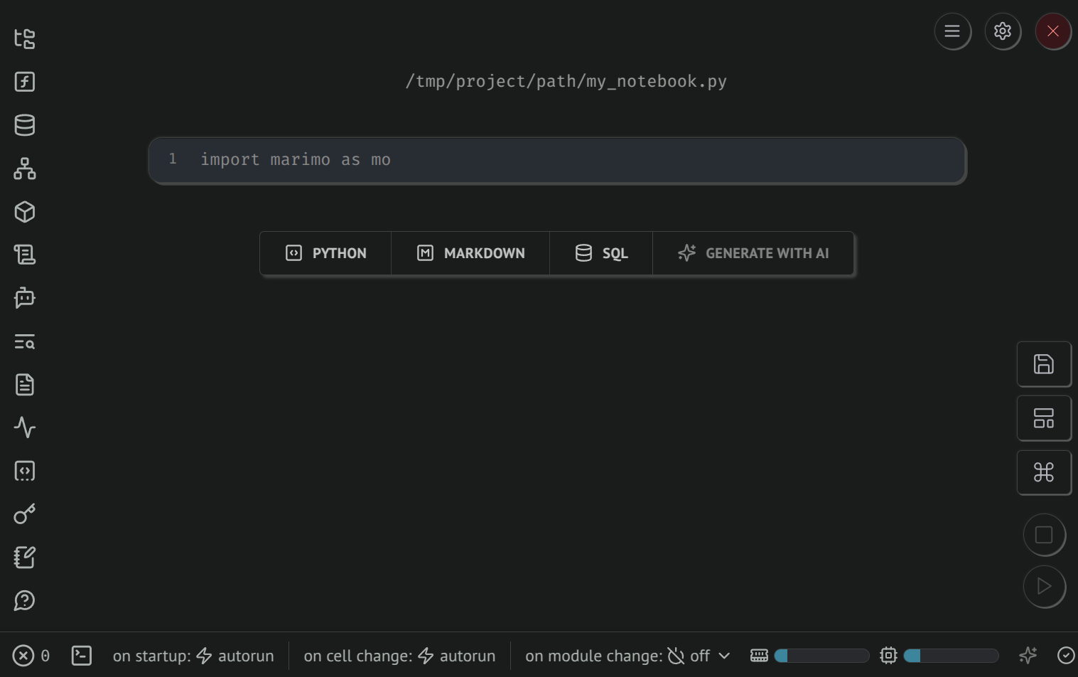
The interface looks like this:

Features

Use custom dlt widgets

Inside your marimo notebook, you can use composable widgets built and maintained by the dlt team. This requires the mowidgets package (Python 3.11+).

Import the widgets from dlt.helpers.marimo. Then pass a widget to the render() function:

#%% cell 1
from dlt.helpers.marimo import render, load_package_viewer, pipeline_selector

#%% cell 2
render(pipeline_selector)

#%% cell 3
render(load_package_viewer, pipeline_path="/path/to/pipeline")

Available widgets: pipeline_selector, load_package_viewer, schema_viewer.

View dataset tables and columns

After loading data with dlt, you can access it via the dataset interface, including a native ibis connection.

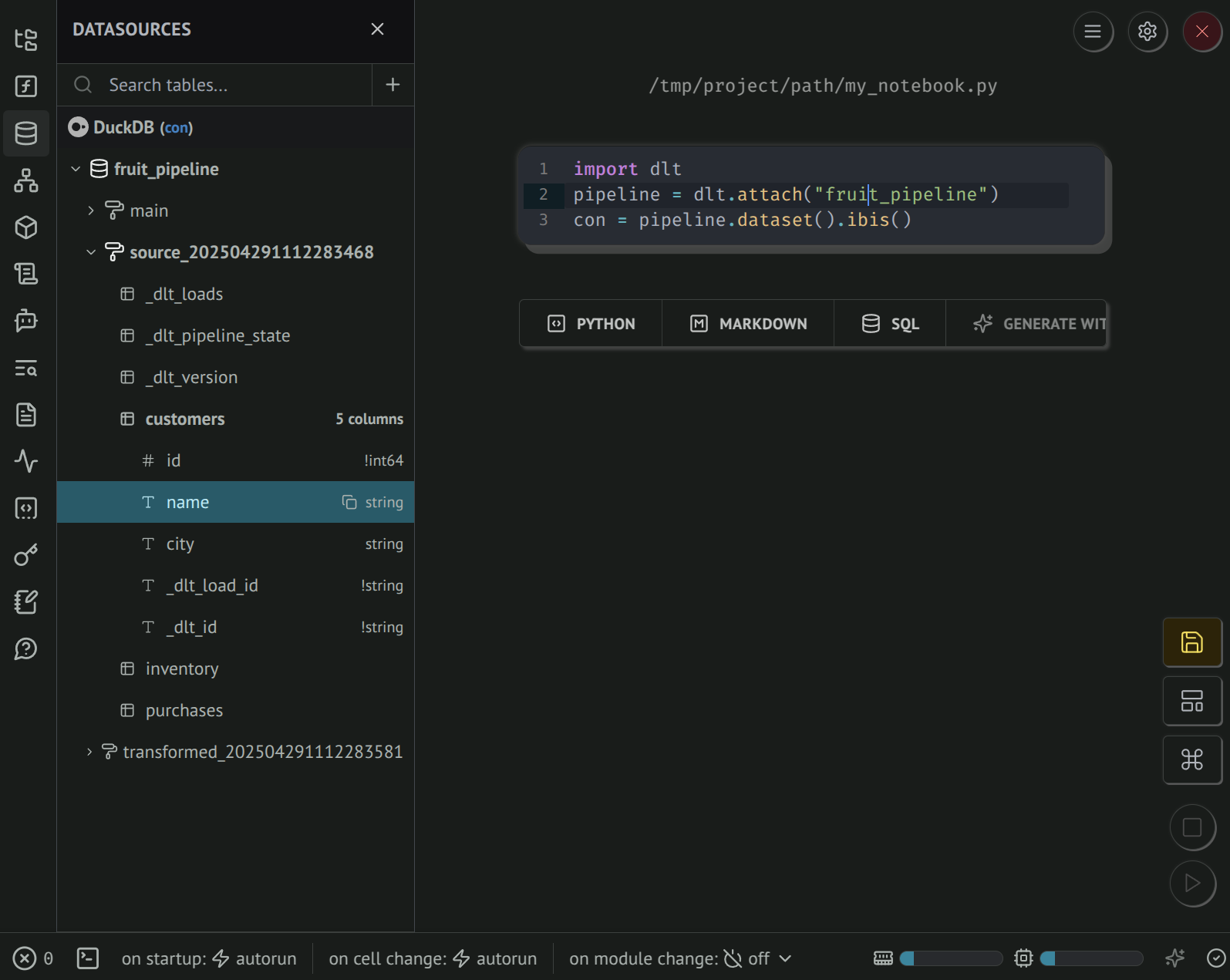
In marimo, the Datasources panel provides a GUI to explore data tables and columns. marimo registers any cell variable that holds an ibis connection.

Access data with SQL

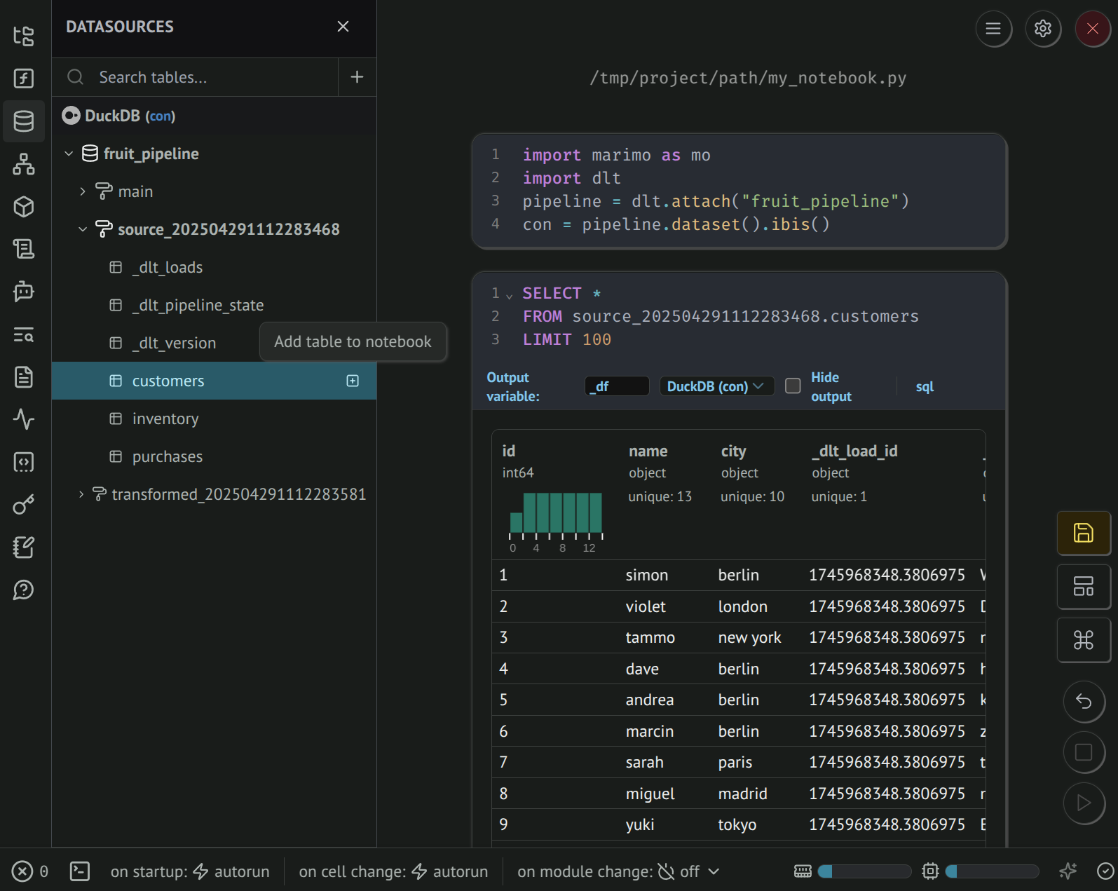
The Add table to notebook button creates a new SQL cell that you can use to query data. The output cell holds an interactive results dataframe.

note

The Datasources panel displays a limited range of data types.

Access data with Python

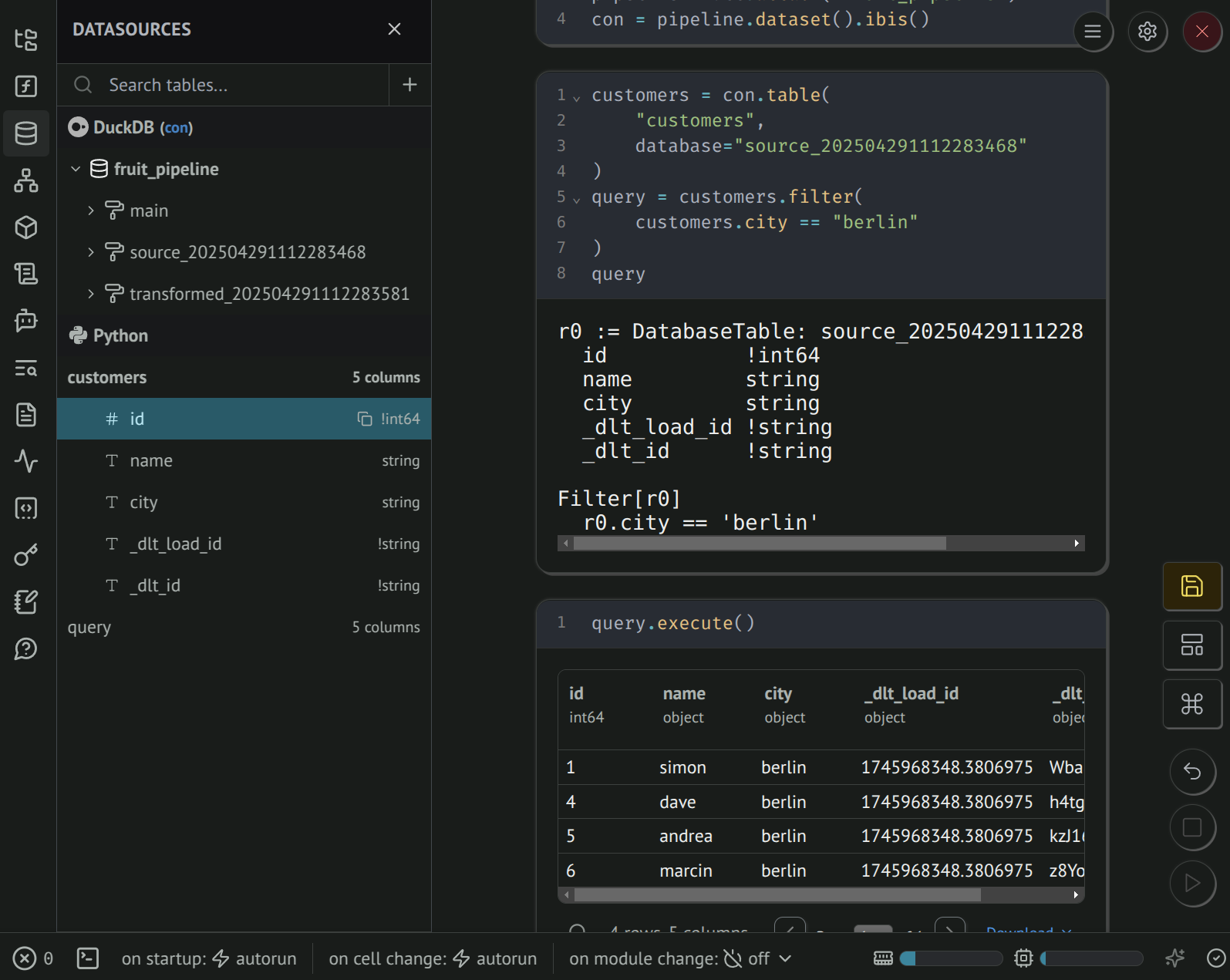
You can also read Ibis tables (deferred expressions) with Python. Under Python, the Datasources panel shows the output schema of your Ibis query. The cell output displays the query plan.

Use .execute(), .to_pandas(), .to_polars(), or .to_pyarrow() to run the Ibis expression. marimo displays the result as an interactive dataframe.

note

The Datasources panel displays a limited range of data types.

Create a dashboard and data apps

You can deploy marimo notebooks as web applications with interactive UI and charts, with the code hidden. Add marimo UI input elements, markdown, and charts from matplotlib, plotly, or altair. Together, dlt, marimo, and ibis build a dashboard on top of fresh data.

Important considerations

Memory usage: A full table read can exhaust memory and stop your program. If a table is large, apply a limit or iterate in chunks.
Deferred reads: Dataset and Relation objects read data only when you take an action that needs it. See Deferred query execution.
Custom SQL queries: limit() and select() do not change a query you wrote yourself. Put every clause you need in the SQL statement.

Quick start example​

Getting started​

Access the dataset​

Access tables as relations​

Create relations with SQL query strings​

Reading data​

Fetch the entire table​

As a Pandas DataFrame​

As a PyArrow Table​

As a list of Python tuples​

Deferred query execution​

Iterating over data in chunks​

Iterate as Pandas DataFrames​

Iterate as PyArrow Tables​

Iterate as lists of tuples​

Connection handling​

Special queries​

Modifying queries​

Limit the number of records​

Using head() to get the first 5 records​

Select specific columns​

Sort results​

Filter rows​

Aggregate data​

Filter to an incremental cursor​

Cursor on an auto-joined column​

Join related tables​

Auto-join via schema references​

Explicit join condition​

Cross-dataset joins​

Cross-destination joins with DuckDB​

Chain operations​

Modifying queries with ibis expressions​

Migrating from the previous dlt / ibis implementation​

Supported destinations​

Reading data from filesystem​

Examples​

Fetch one record as a tuple​

Fetch many records as tuples​

Iterate over data with limit and column selection​

Advanced usage​

Loading a Relation into a pipeline table​

Datasets with multiple schemas​

Breaking changes​

Staging dataset​

dev_mode (versioned datasets)​

Internal dlt tables​

_dlt_loads​

_dlt_pipeline_state​

_dlt_version​

Ibis​

Prerequisites​

Get an Ibis connection from your dataset​

Marimo​

Prerequisites​

Launch marimo​

Features​

Use custom dlt widgets​

View dataset tables and columns​

Access data with SQL​

Access data with Python​

Create a dashboard and data apps​

Further reading​

Important considerations​

DHelp

Ask a question

Quick start example

Getting started

Access the dataset

Access tables as relations

Create relations with SQL query strings

Reading data

Fetch the entire table

As a Pandas DataFrame

As a PyArrow Table

As a list of Python tuples

Deferred query execution

Iterating over data in chunks

Iterate as Pandas DataFrames

Iterate as PyArrow Tables

Iterate as lists of tuples

Connection handling

Special queries

Modifying queries

Limit the number of records

Using `head()` to get the first 5 records

Select specific columns

Sort results

Filter rows

Aggregate data

Filter to an incremental cursor

Cursor on an auto-joined column

Join related tables

Auto-join via schema references

Explicit join condition

Cross-dataset joins

Cross-destination joins with DuckDB

Chain operations

Modifying queries with ibis expressions

Migrating from the previous dlt / ibis implementation

Supported destinations

Reading data from filesystem

Examples

Fetch one record as a tuple

Fetch many records as tuples

Iterate over data with limit and column selection

Advanced usage

Loading a `Relation` into a pipeline table

Datasets with multiple schemas

Breaking changes

Staging dataset

`dev_mode` (versioned datasets)

Internal `dlt` tables

`_dlt_loads`

`_dlt_pipeline_state`

`_dlt_version`

Ibis

Prerequisites

Get an Ibis connection from your dataset

Marimo

Prerequisites

Launch marimo

Features

Use custom dlt widgets

View dataset tables and columns

Access data with SQL

Access data with Python

Create a dashboard and data apps

Further reading

Important considerations