Data monitoring

Data quality monitoring is concerned with ensuring that quality data arrives at the data warehouse on time. The reason we do monitoring instead of alerting for this is because we cannot easily define alerts for what could go wrong.

This is why we want to capture enough context to allow a person to decide if the data looks OK or requires further investigation when monitoring the data quality. A staple of monitoring are line charts and time-series charts that provide a baseline or a pattern that a person can interpret.

For example, to monitor data loading, consider plotting "count of records by loaded_at date/hour", "created at", "modified at", or other recency markers.

Rows count

To find the number of rows loaded per table, use the following command:

dlt pipeline <pipeline_name> trace

This command will display the names of the tables that were loaded and the number of rows in each table. The above command provides the row count for the Chess source. As shown below:

Step normalize COMPLETED in 2.37 seconds.
Normalized data for the following tables:
- _dlt_pipeline_state: 1 row(s)
- payments: 1329 row(s)
- tickets: 1492 row(s)
- orders: 2940 row(s)
- shipment: 2382 row(s)
- retailers: 1342 row(s)

To load this information back to the destination, you can use the following:

# Create a pipeline with the specified name, destination, and dataset
# Run the pipeline

# Get the trace of the last run of the pipeline
# The trace contains timing information on extract, normalize, and load steps
trace = pipeline.last_trace

# Load the trace information into a table named "_trace" in the destination
pipeline.run([trace], table_name="_trace")

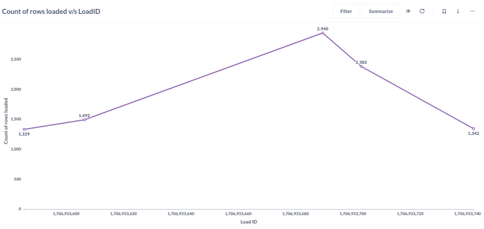
This process loads several additional tables to the destination, which provide insights into the extract, normalize, and load steps. Information on the number of rows loaded for each table, along with the load_id, can be found in the _trace__steps__extract_info__table_metrics table. The load_id is an epoch timestamp that indicates when the loading was completed. Here's a graphical representation of the rows loaded with load_id for different tables:

Data load time

Data loading time for each table can be obtained by using the following command:

dlt pipeline <pipeline_name> load-package

The above information can also be obtained from the script as follows:

info = pipeline.run(source, table_name="table_name", write_disposition='append')

print(info.load_packages[0])

load_packages[0] will print the information of the first load package in the list of load packages.

Tools to create dashboards

Metabase, Looker Studio, Marimo and Streamlit are some common tools that you might use to set up dashboards to explore data. It's worth noting that while many tools are suitable for exploration, different tools enable your organization to achieve different things. Some organizations use multiple tools for different scopes:

• Tools like Metabase are intended for data democratization, where the business user can change the dimension or granularity to answer follow-up questions.
• Tools like Looker Studio and Tableau are intended for minimal interaction curated dashboards that business users can filter and read as-is with limited training.
• Tools like Marimo allow you to build powerful dashboards in the style of iPython notebooks.
• Tools like Streamlit enable powerful customizations and the building of complex apps by Python-first developers, but they generally do not support self-service out of the box.